Frequency Domain

Frequency Transforms

Frequency transforms are classical tools in signal processing where the measurement of spectra is used to characterize time-dependent processes such as speech patterns and radar or sonar data.

Some operations in image processing, such as noise detection and correction, are more effectively carried out in the frequency area. The Fourier transform expresses a function as a sum of sine and cosine components. In the Fast Fourier Transform (FFT) of a 2D (or 3D) image, there are two output images. The frequency information, or module, is stored in an image, while the phase information is stored in another.

The module, or frequency image, is a representation of the frequency of change in pixel values. This allows analysis and processing operations to be executed on the frequency component only.

The phase image contains information about the degree of change in pixel values and is used in combination with the module to reconstruct the image.

The Fourier transform itself is usually only an intermediate step. The algorithms that rely on the Fourier transform fall into three groups:

• Some operations involving periodicity, such as shifting, lineation or blurring, are better represented in the Fourier domain.
• Correlation, convolution, and many linear transformations are more efficiently implemented using the Fourier transform.
• When modified frequencies may be attributed to particular spatial phenomenon, such as noise or transitions, filtering operators or even direct cropping can be used to restore or enhance the image.

Introduction to FFT

The FFT reduces the amount of computation to $N\times \log_2N$ operations instead of the $N^2$ operations involved in a normal Fourier transform.
For images, the classical method consists in computing 1-D FT's successively, since the Fourier transform is separable.
The Fourier transform is computed horizontally and then vertically on the intermediate result: $$ X(u,v)=\frac{1}{N}\sum_{k,l=0}^{N-1} x(k,l) \times e^{-\frac{2i\pi}{N}\times(uk+vl)} $$ $$ X(u,v)=\sum_{k,l} x(k,l) e^{-\frac{2i\pi}{N}\times uk} \times e^{-\frac{2i\pi}{N}\times lv} $$ $$ X(u,v)=\sum_{l} e^{-\frac{2i\pi}{N}\times lv} \left( \sum_{k} x(k,l) e^{-\frac{2i\pi} {N}\times ku} \right) = \sum_{l} e^{-\frac{2i\pi}{N}\times lv} K(u,l) $$ For an image of size $N \times N$, one computes the FT of each line to obtain the functions $K(u, l)$, and then the FT of the $K(u, l)$ along columns. In the discrete case, the Fourier transform of an image is a complex image with a real part and an imaginary part. We usually represent the modulus of the image, and sometimes its phase.
If $X(u, v)$ is the value of a pixel of the FT, we have $X(u,v)=R(u,v)+iI(u,v)$ where $R(u,v)$ is the real part and $I(u,v)$ the imaginary part.
The image of modulus, called the spectrum is defined as: $$ M(u,v) = \sqrt{R^2(u,v)+I^2(u,v)} $$ and the phase image as: $$ \Phi(u,v) = A\tan(\frac{I(u, v)}{R(u,v)}) $$ The Fourier transform may be written using an exponential notation: $$ X(u,v)=M(u,v) \times \exp(-2i\pi\Phi(u,v)) $$ The modulus is centered: the frequency (0,0) is placed at the center of the image. A negative frequency -u corresponds to the positive N-u frequency: $$ e^{-\frac{2i\pi(-u)k}{N}}=e^{-\frac{2i\pi(N-k)}{N}} $$ The modulus at point (0,0) is proportional to the mean of the image and has no significance from the frequency point of view. The transform usually has large values in the vicinity of the center and very low values elsewhere. This unequal dynamic distribution may make it necessary to transform the modulus to see it better. One must be careful that high values do not hide low ones.

Some suggest the use of the logarithm of the modulus for display; others, histogram equalization. It is also possible to stretch the histogram between two given bounds (including 95$\%$ of the pixels, for example), and clamp the values outside the range.

Examples of Fourier Transforms

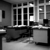
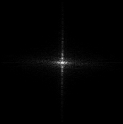
The modulus image has usually a rather isotropic central halo shape with a cross made of the central column and row. This image uniformity, except when particular structures are present, makes the modulus interpretation rather difficult, as shown in Figure 1.

Figure 1. An image and its Fourier transform modulus

Impulse image

An impulse image is an image with zero values everywhere except for one location. The image is reduced to a single point:

• $ x(k_0, l_0) = a $
• $ x(k, l) = 0 $ everywhere else.

The discrete Fourier transform of a point is the complex constant: $$ X(u,v)=\frac{a}{N} \times e^{-\frac{2i\pi}{N}\times(uk_0+vl_0)} $$ $$ |X(u,v)|=\frac{|a|}{N} \times \left | e^{-\frac{2i\pi}{N}\times(uk_0+vl_0)} \right | = \frac{|a|}{N} $$ The modulus is constant and the spectrum is uniform.

Constant image

For a constant image, for instance $x(k,l) = a$ for all k and l, the discrete Fourier transform is an image where only the frequency located at (0,0) in the Fourier space is non-zero: $$ X(u,v)=\frac{a}{N}\sum_{k,l=0}^{N-1} e^{-\frac{2i\pi}{N}\times(uk+vl)} $$ Thus: $$ \left\{\begin{array}{ll} X(0,0) = \frac{a}{N}\times N^2 \\ X(u,v) = \frac{a}{N} \times 0 = 0 & \mbox{elsewhere} \end{array}\right. $$

Parallel lines

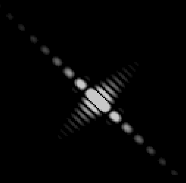
The function $cos(ux+vy)$ corresponds to waves perpendicular to the $(u,v)$ direction. The corresponding image looks like a succession of black and white stripes. The distance between two successive black (or white) strips is $ \sqrt{u^2+v^2}$.
The discrete Fourier transform is zero everywhere except at $(u, v)$ and $(-u, -v)$. Spectral analysis corresponds here to the intuitive notion that the Fourier transform of a base function of the Fourier space is reduced to a Dirac impulse function.

More generally, successive parallel lines of frequency $(u,v)$ have a Fourier transform with two peaks at location $(u,v)$ and $(-u,-v)$.
The peaks indicate the base frequency of the pattern. Real images rarely match a perfect model, but rather come close to a particular model that the Fourier transform can highlight.

Two possible reasons for deviation from a particular model are:

• If the pattern is not absolutely straight but exhibits a slight curving (such as fringes of interference for instance), peaks are not points anymore but are spread out over a surface whose spread and slant are related to the amount of curving in the lines.
• If the pattern is not really periodic or if it is noisy, a halo appears around the main frequency. The Fourier transform shows the general direction of the pattern, and sometimes its main frequency, which are not usually easy to determine on the spatial domain image.

Periodic structures

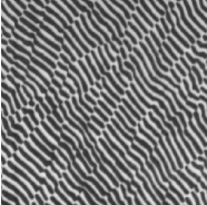
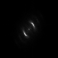
The FFT can help to quantify a linear periodic structure. Figure 2 is an electron microscope view of fibers in a metal sample. The goal is to find their orientation and periodicity. The segments are not truly parallel, and the sections within the structure generate circular arcs around the base frequency in the Fourier spectrum image.

Figure 2. Periodic structure and its FFT modulus

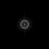
Edges or transitions

If an image contains an edge, or a transition along a line of orientation $ \theta $, its Fourier spectrum shows a line intersecting the center of the image with the orientation $ \theta + \pi /2 $, as in Figure 3. Along this line, the Fourier coefficients are larger than their neighbors.

Figure 3. Transition along a line
This explains the cross through the center of the Fourier spectrum. Since the image wraps around, the last and first columns, and the last and first lines are neighbors which may cause high-frequency artifacts to appear on the spectrum. These artifacts are absent if the values are not significantly different from the real transitions between rows or columns.

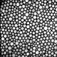
Networks

In an image made up of cells or objects partitioning the image, as in Figure 4, the FFT illustrates the presence of a network. Two cells are at a mean distance equal to $d$. If the distribution is stationary (the density is constant in each subarea of the image, the cells have similar shapes) and isotropic (no privileged direction), the modulus of the Fourier transform is a bright ring centered in (0,0), of radius $N/d$ where $N$ is equal to the size of the image. The central cross is almost invisible in this case.

Figure 4. Networks or cell structures

Shifting

Shifting can be detected between two similar and highly correlated images, translated one from the other by a vector $(a,b)$. This situation is frequent in the following situations:

• Motion study in a gas.
• Trajectory analysis.
• Remote sensing applications, where the two images are taken by two scanners slightly shifted.

The modulus of the difference of the Fourier transforms exhibits fringes, similar to interference fringes, in the directions $(a,b)$ and with a distance of: $$ \frac{N}{\sqrt{a^2+b^2}} $$ If sub-pixels shift, one must look at the difference of phase images. The shift appears as a plane whose equation is directly linked to the amount of the shift.

Figure 5. Gas image and its Fourier Transform

Periodicity

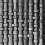
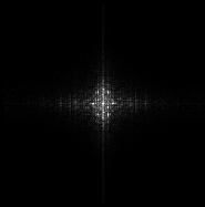
Usually, periodicities stand out in the FFT. We already saw the case of parallel lines. More complex cases remain very close to that ideal situation.
For instance, considering the Fourier transform of an image of vertical parallel camshafts in Figure 6, the horizontal periodicity of the camshafts generates two peaks on the horizontal axis. The two symmetric peaks correspond to parallel and interrupted horizontal lines of the cams and spaced by an average distance of 21 pixels. For a 256x256 image, peaks are then at frequencies of $ \pm 256/21 = \pm 12$.
Other peaks are more difficult to interpret and result from periodic structures in the cams, in certain directions (vertical for example).

Figure 6. Camshafts and their FFT