Moments And Orientations
Analysis algorithms measuring features globally to the input image based on moments of inertia and covariance matrices.
- MomentsOfInertia2d: Computes the elements of the covariance matrix of a two-dimensional grayscale image.
- MomentsOfInertia3d: Computes the elements of the covariance matrix of a three-dimensional grayscale image.
- InertiaMoment2d: Measures the resistance of an object, defined by a two-dimensional binary image, to changes in its motion around a given axis of rotation.
- Eccentricity2d: Computes a shape factor of a binary two-dimensional image.
- OrientationMapFourier3d: Determines a block-wise orientation of structures contained in a three-dimensional grayscale image.
- OrientationMatchingFourier3d: Estimates the probability of a sample to be locally oriented in a user-defined direction.
These measurements are useful for determining the global characteristics of a shape.
Notice: Some parts of the following information is only relevant for some individual measurements available with the LabelAnalysis algorithm.
In the continuous case they are defined as: $$ M_{1x}=\frac{1}{A(X)}\int_X x \times g(x,y,z) \, dx \, dy \, dz $$ $$ M_{1y}=\frac{1}{A(X)}\int_X y \times g(x,y,z) \, dx \, dy \, dz $$ $$ M_{1z}=\frac{1}{A(X)}\int_X z \times g(x,y,z) \, dx \, dy \, dz $$ and in the discrete case as: $$ M_{1x} = \frac{1}{A(X)}\sum_{X}{x_i \times g(x_i,y_j,z_k)} $$ $$ M_{1y} = \frac{1}{A(X)}\sum_{X}{y_j \times g(x_i,y_j,z_k)} $$ $$ M_{1z} = \frac{1}{A(X)}\sum_{X}{z_k \times g(x_i,y_j,z_k)} $$ where:
Notes:
In an elongated ellipsoid, the largest eigenvalue expresses the longest axis.
In ImageDev, the index convention is:
This is a good measure of orientation for simple and roughly convex objects.
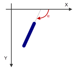
Figure 1. 2D convention for defining an orientation (alpha angle)
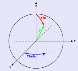
Figure 2. Azimuthal and polar angles on the unit sphere
These values indicate the extents of the bounding box of the shape oriented along the corresponding eigenvector, with respect to the barycenter (maximal extents are positive, minimal extents are negative).
A disk or a cross has a null eccentricity as $\lambda_1=\lambda_2$. The eccentricity increases with the difference between the eigenvalues, and thus measures the elongation of the object.
It also indicates in some cases a privileged direction, corresponding to a large eigenvalue and a small one; for instance, $(\lambda_1-\lambda_2)^2$ has a high value, though two orthogonal privileged directions mean two large eigenvalues and a smaller difference $(\lambda_1-\lambda_2)^2$.
Notice: Some parts of the following information is only relevant for some individual measurements available with the LabelAnalysis algorithm.
First order moments
The first order moments define the centroid or center of mass or barycenter.In the continuous case they are defined as: $$ M_{1x}=\frac{1}{A(X)}\int_X x \times g(x,y,z) \, dx \, dy \, dz $$ $$ M_{1y}=\frac{1}{A(X)}\int_X y \times g(x,y,z) \, dx \, dy \, dz $$ $$ M_{1z}=\frac{1}{A(X)}\int_X z \times g(x,y,z) \, dx \, dy \, dz $$ and in the discrete case as: $$ M_{1x} = \frac{1}{A(X)}\sum_{X}{x_i \times g(x_i,y_j,z_k)} $$ $$ M_{1y} = \frac{1}{A(X)}\sum_{X}{y_j \times g(x_i,y_j,z_k)} $$ $$ M_{1z} = \frac{1}{A(X)}\sum_{X}{z_k \times g(x_i,y_j,z_k)} $$ where:
- $(x_i,y_j,z_k)$ is a point of the object $X$.
- $g$ its gray level intensity.
- $A(X)$ the area of $X$.
Notes:
- The names of ImageDev measurements based on these computations start with Gray if the moments are computed weighting the result by the gray levels of the intensity image (for example, GrayBarycenterX).
- Other moment-based measurements do not take into account the gray levels of the intensity image (for example, BarycenterX).
- If the intensity image given to the analysis algorithm is a binary image, both types of measurement will output the same result ( GrayBarycenterX = BarycenterX).
Second order moments
The second order moments are defined in the discrete case as: $$ M_{2x} = \frac{1}{A(X)}\sum_{X}{(x_i-M_{1x})^2 \times g(x_i,y_j,z_k)} $$ $$ M_{2y} = \frac{1}{A(X)}\sum_{X}{(y_i-M_{1y})^2 \times g(x_i,y_j,z_k)} $$ $$ M_{2z} = \frac{1}{A(X)}\sum_{X}{(z_i-M_{1z})^2 \times g(x_i,y_j,z_k)} $$ $$ M_{2xy} = \frac{1}{A(X)}\sum_{X}{(x_i-M_{1x})(y_i-M_{1y}) \times g(x_i,y_j,z_k)} $$ $$ M_{2xz} = \frac{1}{A(X)}\sum_{X}{(x_i-M_{1x})(z_i-M_{1z}) \times g(x_i,y_j,z_k)} $$ $$ M_{2yz} = \frac{1}{A(X)}\sum_{X}{(y_i-M_{1y})(z_i-M_{1z}) \times g(x_i,y_j,z_k)} $$Variance-covariance matrix
The covariance matrix (or variance-covariance matrix) of a 2D image can be written as: $$ M = \begin{bmatrix} M_{2x} & M_{2xy}\\ M_{2xy} & M_{2y}\end{bmatrix} $$ and for a 3D image: $$ M= \begin{bmatrix} M_{2x} & M_{2xy} & M_{2xz}\\ M_{2xy} & M_{2y} & M_{2yz}\\ M_{2xz} & M_{2yz} & M_{2z}\end{bmatrix} $$Eigenvalues and eigenvectors
The eigenvalues and eigenvectors are computed by performing a Singular Value Decomposition (SVD) of the covariance matrix.In an elongated ellipsoid, the largest eigenvalue expresses the longest axis.
In ImageDev, the index convention is:
- Index 1 refers to the largest eigenvalue and its associated eigenvector.
- Index 2 refers to the medium eigenvalue and its associated eigenvector in 3D and to the smallest in 2D.
- Index 3 refers to the smallest eigenvalue and its associated eigenvector in 3D.
Orientations
The main orientation of a shape is defined as the direction of its major inertia axis. It is given by the eigenvector of the largest eigenvalue of the covariance matrix.This is a good measure of orientation for simple and roughly convex objects.
2D orientations
In 2D, the orientation is given by a single value representing the angle between the X axis and the eigenvector. This angle falls between -90 and 90 degrees.Figure 1. 2D convention for defining an orientation (alpha angle)
3D orientations
In 3D, the orientations are given by the spherical coordinates ($\theta$, $\varphi$), as often used in mathematics (azimuthal angle, $\theta$ and polar angle, $\varphi$). The relation between eigenvector and orientation is given by the following formula: $$V=\begin{bmatrix} v_x\\ v_y\\ v_z\end{bmatrix} = \begin{bmatrix} \sin(\varphi)\cos(\theta)\\ \sin(\varphi)\sin(\theta)\\ \cos(\varphi)\end{bmatrix}$$ This direction can be illustrated on the unit sphere:Figure 2. Azimuthal and polar angles on the unit sphere
- The result $\theta$ falls between -180 and +180 degrees.
- The result $\varphi$ falls between 0 and 90 degrees.
Extent values
The extent of the data can be computed in the direction of the largest, medium, and smallest eigenvectors of the covariance matrix.These values indicate the extents of the bounding box of the shape oriented along the corresponding eigenvector, with respect to the barycenter (maximal extents are positive, minimal extents are negative).
Eccentricity
The eccentricity of a 2D image is defined as: $$E_c(X) = (4\pi)^2\frac{(\lambda_1-\lambda_2)^2}{A^2(X)} = (4\pi)^2\frac{(M_{2x}-M_{2y})^2+4M^2_{2xy}}{A^2(X)}$$ $\lambda_1$ and $\lambda_2$ are the covariance matrix eigenvalues.A disk or a cross has a null eccentricity as $\lambda_1=\lambda_2$. The eccentricity increases with the difference between the eigenvalues, and thus measures the elongation of the object.
It also indicates in some cases a privileged direction, corresponding to a large eigenvalue and a small one; for instance, $(\lambda_1-\lambda_2)^2$ has a high value, though two orthogonal privileged directions mean two large eigenvalues and a smaller difference $(\lambda_1-\lambda_2)^2$.