Mathematical Morphology
This category introduces a theory for the analysis of geometrical structures.
- Erosion And Dilation: Morphological erosion and dilation algorithms.
- Opening And Closing: Morphological opening and closing algorithms.
- Hit Or Miss And Skeleton: Algorithms computing morphological skeleton and applying post-processing on it.
- Geodesic Transformations: Algorithms based on geodesic propagations such as reconstructions.
- Distance Maps: Algorithms computing geodesic metrics on binary images.
Morphology is based on the use of set operators (intersection, union, inclusion, complement) to transform an
image. The transformed image usually has fewer details, implying a loss of information, but its main
characteristics are still present. Once an image has been simplified by morphological processing, measurements can
be computed to provide a quantitative analysis of the image.
The basic morphological operators are either erosions or dilations. ImageDev supports several types of erosions and dilations such as: Erosion2d, ErosionDisk2d, ErosionBall3d, ErosionLine2d, ErosionColor2d, Dilation2d, DilationDisk2d, DilationBall3d, DilationLine2d and DilationColor2d.
There are two types of morphological transformations: regular and recursive. In a regular morphological transformation, the structuring element examines the pixel values in the original image to establish the new pixel value. In a recursive morphological transformation, the new values established by the structuring element are affected by the previously changed values. Regular morphological transformations are obviously more accurate, but require more time to compute.
Alternatively, a point may have 4 neighbors, and a basic structuring element is then a cross:
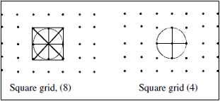
Figure 1. Structuring elements
The central voxel (in red in Figure 2) may have 26 neighbors, and a basic structuring element is a cube.
Alternatively a point may have 6 neighbors (voxels in green), and a basic structuring element is then a cross.
A point may also have 18 neighbors.
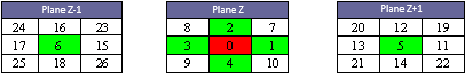
Figure 2. Structuring elements: cube with 26 neighbors (white and green) or cross with 6 neighbors (green)
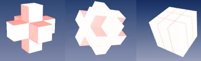
Figure 3. Structuring elements: 6-neighbors (left), 18-neighbors (middle) and 26- neighbors (right)
The basic morphological operators are either erosions or dilations. ImageDev supports several types of erosions and dilations such as: Erosion2d, ErosionDisk2d, ErosionBall3d, ErosionLine2d, ErosionColor2d, Dilation2d, DilationDisk2d, DilationBall3d, DilationLine2d and DilationColor2d.
Structuring Elements
Morphological transformation is based on a structuring element $(B)$ characterized by shape, size, and location of its center. Each pixel in an image is compared with $B$ by moving $B$ so that its center hits the pixel. Depending on the type of morphological transformation, the pixel value is reset to the value or average value of one or more of its neighbors.There are two types of morphological transformations: regular and recursive. In a regular morphological transformation, the structuring element examines the pixel values in the original image to establish the new pixel value. In a recursive morphological transformation, the new values established by the structuring element are affected by the previously changed values. Regular morphological transformations are obviously more accurate, but require more time to compute.
Mathematical Morphology on 2D images
On a square grid, a point may have 8 neighbors, in which case a basic structuring element is a square.Alternatively, a point may have 4 neighbors, and a basic structuring element is then a cross:
Figure 1. Structuring elements
Mathematical Morphology on 3D images
The central voxel (in red in Figure 2) may have 26 neighbors, and a basic structuring element is a cube.
Alternatively a point may have 6 neighbors (voxels in green), and a basic structuring element is then a cross.
A point may also have 18 neighbors.
Figure 2. Structuring elements: cube with 26 neighbors (white and green) or cross with 6 neighbors (green)
Figure 3. Structuring elements: 6-neighbors (left), 18-neighbors (middle) and 26- neighbors (right)
Type of connectivity
For algorithms supporting several connectivity types, the neighbor configuration can be set with a neighborhood parameter (for example, in Dilation3d).© 2026 Thermo Fisher Scientific Inc. All rights reserved.