Geometry
Contains measurements expressing shape attributes.
Note: These measurements ignore the intensity input image.
For example, consider a set of lines $d(X,\alpha)$, parallel to a direction $\alpha$ and regularly spaced by $dx$.
The diametral variation is defined as: $$D_2(X,\alpha)=\int{N_\alpha(X)dx}$$ Where $N_\alpha(X)$ is the number of boundary points that intersect the set of lines $d(x,\alpha)$. This is equivalent to the sum of the lengths of the projections of the object in the $\alpha$ direction. Note that $D_2(X,\alpha)$ is symmetric:
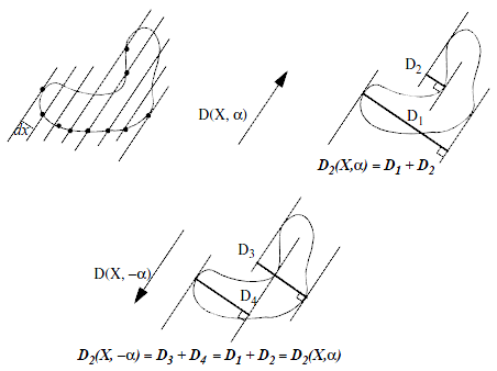
Figure 1. Application of the diametral variation formula
The discrete case in 2D translates to the search for specific configurations, as defined in the following table. $$ \begin{array}{|c|c|c|c|c|} \hline Orientation & 0^\circ & 45^\circ & 90^\circ & 135^\circ\\ \hline Kernel & \begin{array}{ccc} \mbox{x} & \mbox{x} & \mbox{x}\\ \mbox{x} & 0 & 1\\ \mbox{x} & \mbox{x} & \mbox{x} \end{array} & \begin{array}{ccc} \mbox{x} & \mbox{x} & 1\\ \mbox{x} & 0 & \mbox{x}\\ \mbox{x} & \mbox{x} & \mbox{x} \end{array} & \begin{array}{ccc} \mbox{x} & 1 & \mbox{x}\\ \mbox{x} & 0 & \mbox{x}\\ \mbox{x} & \mbox{x} & \mbox{x} \end{array} & \begin{array}{ccc} 1 & \mbox{x} & \mbox{x}\\ \mbox{x} & 0 & \mbox{x}\\ \mbox{x} & \mbox{x} & \mbox{x} \end{array}\\ \hline \end{array}$$
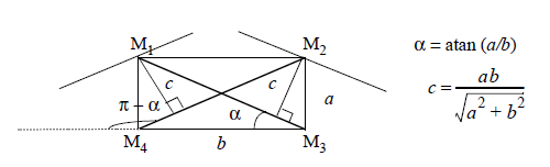
Figure 2. Crofton perimeter on non-square pixels
The formula becomes:
$$ L(X)=\alpha \times a \times N_0 + (\frac{\pi}{2}-\alpha)\times b \times N_{90} + \frac{\pi}{4}\times c
\times (N_{\alpha}+N_{\pi-\alpha}) $$
Let's consider a disk with a diameter of 11 pixels, as shown in Figure 3, and a pixel size equal to (1, 1).
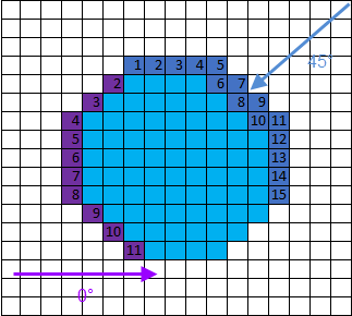
Figure 3. Computation of the Crofton perimeter on a disk
Then we have:
The theoretical value is deduced from the diameter ($\pi \times D$). While it is given here as reference, it should not be considered as an absolute truth because of discretization issues when building the disks. The error percentage of each measurement is computed as follows: $$ Error = 100 \times \frac {\left| Theoretical - Measurement \right| }{Theoretical} $$ $$ \begin{array}{|c||c|c|c|c|} \hline \textbf{Diameter} & \textbf{Theoretical} & \textbf{Boundary (Error %)} & \textbf{Crofton (Error %)}& \textbf{Segment (Error %)} \\ \hline \hline 3 & 9.42 & 5~(46.9) & 8.04~(14.6) & 7.11~(24.5) \\ \hline 11 & 34.56 & 40~(15.7) & 33.94~(1.8) & 34.69~(0.4) \\ \hline 31 & 97.39 & 116~(19.1) & 96.46~(1.0) & 95.99~(1.4) \\ \hline 55 & 172.79 & 212~(22.7) & 171.92~(0.5) & 172.72~(0.0) \\ \hline 99 & 311.02 & 388~(24.8) & 309.~(0.4) & 311.39~(0.1) \\ \hline 203 & 637.74 & 804~(26.1) & 635.43.~(0.4) & 343.29~(0.9) \\ \hline \end{array} $$ $$ \begin{matrix} \textbf{Table 1. }\text{Comparison between theoretical perimeter, boundary pixel count,} \\ \text{Crofton Perimeter, and polygonal aproximation perimeter on a synthetic disk} \\ \end{matrix} $$
A better estimation consists of extending the Crofton perimeter concept to the 3D area by computing diametral variations in 13 directions and summing these values with weights appropriate to each direction. This estimation is less sensitive to orientation or surface roughness than the previous method. It is especially imprecise for objects made of few voxels.
The table below presents the surface area values computed by ImageDev on synthetic spheres of different diameters $D$. All values are expressed in pixels for convenience, however they could be computed in calibration unit.
The theoretical value is deduced from the diameter ($\pi \times D^2$). While it is given here as reference, it should not be considered as an absolute truth because of discretization issues when building the spheres.
$$ \begin{array}{|c||c|c|c|} \hline \textbf{Diameter} & \textbf{Theoretical} & \textbf{Voxel Face (Error %)} & \textbf{Area3d (Error %)} \\ \hline \hline 3 & 28.27 & 54~(91.0) & 41.07~(45.3) \\ \hline 11 & 380.13 & 606~(59.4) & 427.12~(12.4) \\ \hline 31 & 3019.07 & 4662~(54.4) & 3138.37~(4.0) \\ \hline 55 & 9503.31 & 14406~(51.6) & 9700.41~(2.1) \\ \hline 99 & 30790.72 & 46518~(51.1) & 31127.94~(1.1) \\ \hline 203 & 129~461.78 & 194~742~(50.4) & 130~066.49~(0.5) \\ \hline \end{array} $$ $$ \textbf{Table 2. }\text{Comparison between theoretical surface area, voxel face area, and Crofton area on a synthetic sphere} $$
See related example
Note: These measurements ignore the intensity input image.
Intercepts and diametral variation
Several geometric measurements, such as the Crofton perimeter, and the 3D area, are approximations based on the diametral variation concept.For example, consider a set of lines $d(X,\alpha)$, parallel to a direction $\alpha$ and regularly spaced by $dx$.
The diametral variation is defined as: $$D_2(X,\alpha)=\int{N_\alpha(X)dx}$$ Where $N_\alpha(X)$ is the number of boundary points that intersect the set of lines $d(x,\alpha)$. This is equivalent to the sum of the lengths of the projections of the object in the $\alpha$ direction. Note that $D_2(X,\alpha)$ is symmetric:
Figure 1. Application of the diametral variation formula
The discrete case in 2D translates to the search for specific configurations, as defined in the following table. $$ \begin{array}{|c|c|c|c|c|} \hline Orientation & 0^\circ & 45^\circ & 90^\circ & 135^\circ\\ \hline Kernel & \begin{array}{ccc} \mbox{x} & \mbox{x} & \mbox{x}\\ \mbox{x} & 0 & 1\\ \mbox{x} & \mbox{x} & \mbox{x} \end{array} & \begin{array}{ccc} \mbox{x} & \mbox{x} & 1\\ \mbox{x} & 0 & \mbox{x}\\ \mbox{x} & \mbox{x} & \mbox{x} \end{array} & \begin{array}{ccc} \mbox{x} & 1 & \mbox{x}\\ \mbox{x} & 0 & \mbox{x}\\ \mbox{x} & \mbox{x} & \mbox{x} \end{array} & \begin{array}{ccc} 1 & \mbox{x} & \mbox{x}\\ \mbox{x} & 0 & \mbox{x}\\ \mbox{x} & \mbox{x} & \mbox{x} \end{array}\\ \hline \end{array}$$
2D perimeter of object boundary
Three measurements are available in ImageDev for assessing perimeters:- BoundaryPixelCount: It is simply the number of foreground pixels connected to the background. As it tends to overestimate the perimeter and does not consider the pixels size, it is not recommended to use this method for assessing a perimeter.
- CroftonPerimeter2d: It sums the "seen perimeter" under four different orientations. This method is explained in more detail in the following paragraph.
- PolygonePerimeter2d: It is the cumulated length of the segments provided by polygonal approximation. This estimator gives good results for shapes with smooth boundaries but can miss information on rough boundaries. This measurement is part of the Segment category.
Crofton perimeter
The Crofton formula computes the perimeter using the intercept count. Cauchy's formula shows that: $\alpha$, and regularly spaced by $dx$. $$L(X)=\int_{0}^{\pi}D_2(X,\alpha)d\alpha$$ The perimeter is then approximated when the above integral is replaced by a discrete summation. In the square grid case, the summation is computed for the four fundamental directions: $$ L(X)=\frac{\pi}{4}\times [a \times(N_0+N_{90})+\frac{a}{\sqrt2}\times(N_{45}+N_{135})] $$ Where:- $N_\alpha$ represents the intercept count along the direction $\alpha$,
- $a$ represents the distance between two points on the grid and the distance between two lines in the $0^\circ$ or $90^\circ$ directions,
- $\frac{a}{\sqrt2}$ is the distance between two lines in the $45^\circ$ and $135^\circ$ directions.
Figure 2. Crofton perimeter on non-square pixels
Figure 3. Computation of the Crofton perimeter on a disk
- $a = b = 1$
- $N_0 = N_{90} = 11$
- $N_{45} = N_{135} = 15$
- $L(X) = \frac{\pi}{4}\times \left(2 \times 11 +\frac{2 \times 15}{\sqrt2}\right)$
- $L(X) = 33.94$
Comparison of perimeter estimators
The table below presents the perimeter values computed by ImageDev on synthetic disks of different diameters $D$. All values are expressed in pixels for convenience. All these results could be computed in calibration unit, except the boundary pixel count which is a number of pixels.The theoretical value is deduced from the diameter ($\pi \times D$). While it is given here as reference, it should not be considered as an absolute truth because of discretization issues when building the disks. The error percentage of each measurement is computed as follows: $$ Error = 100 \times \frac {\left| Theoretical - Measurement \right| }{Theoretical} $$ $$ \begin{array}{|c||c|c|c|c|} \hline \textbf{Diameter} & \textbf{Theoretical} & \textbf{Boundary (Error %)} & \textbf{Crofton (Error %)}& \textbf{Segment (Error %)} \\ \hline \hline 3 & 9.42 & 5~(46.9) & 8.04~(14.6) & 7.11~(24.5) \\ \hline 11 & 34.56 & 40~(15.7) & 33.94~(1.8) & 34.69~(0.4) \\ \hline 31 & 97.39 & 116~(19.1) & 96.46~(1.0) & 95.99~(1.4) \\ \hline 55 & 172.79 & 212~(22.7) & 171.92~(0.5) & 172.72~(0.0) \\ \hline 99 & 311.02 & 388~(24.8) & 309.~(0.4) & 311.39~(0.1) \\ \hline 203 & 637.74 & 804~(26.1) & 635.43.~(0.4) & 343.29~(0.9) \\ \hline \end{array} $$ $$ \begin{matrix} \textbf{Table 1. }\text{Comparison between theoretical perimeter, boundary pixel count,} \\ \text{Crofton Perimeter, and polygonal aproximation perimeter on a synthetic disk} \\ \end{matrix} $$
3D area of object boundary
Computing the area of a 3D object boundary is not a trivial issue. An intuitive idea would be to sum the area of voxel faces connected to the background. If it gives a relevant response for objects made of few voxels or perfect axis-aligned cubes, it tends to overestimate the area, especially for uneven surfaces.A better estimation consists of extending the Crofton perimeter concept to the 3D area by computing diametral variations in 13 directions and summing these values with weights appropriate to each direction. This estimation is less sensitive to orientation or surface roughness than the previous method. It is especially imprecise for objects made of few voxels.
The table below presents the surface area values computed by ImageDev on synthetic spheres of different diameters $D$. All values are expressed in pixels for convenience, however they could be computed in calibration unit.
The theoretical value is deduced from the diameter ($\pi \times D^2$). While it is given here as reference, it should not be considered as an absolute truth because of discretization issues when building the spheres.
$$ \begin{array}{|c||c|c|c|} \hline \textbf{Diameter} & \textbf{Theoretical} & \textbf{Voxel Face (Error %)} & \textbf{Area3d (Error %)} \\ \hline \hline 3 & 28.27 & 54~(91.0) & 41.07~(45.3) \\ \hline 11 & 380.13 & 606~(59.4) & 427.12~(12.4) \\ \hline 31 & 3019.07 & 4662~(54.4) & 3138.37~(4.0) \\ \hline 55 & 9503.31 & 14406~(51.6) & 9700.41~(2.1) \\ \hline 99 & 30790.72 & 46518~(51.1) & 31127.94~(1.1) \\ \hline 203 & 129~461.78 & 194~742~(50.4) & 130~066.49~(0.5) \\ \hline \end{array} $$ $$ \textbf{Table 2. }\text{Comparison between theoretical surface area, voxel face area, and Crofton area on a synthetic sphere} $$
See related example
Object members
| Measurement name | Description | Element type | Indexing | Physical Information |
|---|---|---|---|---|
| PixelCount | The number of voxels of a 3D object or pixels of a 2D object. | Integer | [label] | COUNT |
| Area2d | The area of a 2D object, expressed in the image calibration unit.
More information is available in the Area2d algorithm documentation. |
Floating point | [label] | AREA |
| EquivalentDiameter | The diameter of the circular particle of same area in 2D, of the spherical particle of same volume in 3D. It is expressed in the image calibration unit.
|
Floating point | [label] | LENGTH |
| CroftonPerimeter2d | For each of the 8 intercept measurements, the diametral variation is the product of the intercept with the distance between interception points. The Crofton perimeter is the average of those 8 diametral variation measurements, expressed in the image calibration unit.
More information is available in the Intercept count and Crofton Perimeter sections. |
Floating point | [label] | LENGTH |
| BoundaryPixelCount | The number of boundary voxels of a 3D object or pixels of a 2D object; that is, the number of foreground elements that are neighbors of at least one background element. | Integer | [label] | COUNT |
| Volume3d | The volume of a 3D object, expressed in the image calibration unit. | Floating point | [label] | VOLUME |
| Area3d | The 3D area of the object boundary, expressed in the image calibration unit. This measurement uses "intercepts" to take into account the exposed surface of the outer voxels. The idea being that in the "corners", the contribution of a voxel can vary from 1 to 3 depending on configuration.
More information is available in the Intercept count and 3D area of object boundary sections. |
Floating point | [label] | AREA |
| VoxelFaceArea3d | The sum of voxel surfaces that are on the outside of each connected component, expressed in the image calibration unit.
More information is available in the 3D area of object boundary section. |
Floating point | [label] | RATIO |
| VolumeFraction | The ratio between the object area or volume and the total image area or volume.
|
Floating point | [label] | FRACTION |
| InverseCircularity2d | The inverse circularity shape factor, close to 1 for a disk, and greater for star-shaped objects.
The formula to compute this factor is: $$ \frac{CroftonPerimeter2d^2}{4\pi \times Area2d} $$ |
Floating point | [label] | RATIO |
| InverseSphericity3d | The inverse sphericity shape factor, close to 1 for a ball, and greater for tortuous boundary objects.
The formula to compute this factor is: $$ \frac{Area3d^3}{36\pi \times Volume3d^2} $$ |
Floating point | [label] | RATIO |
| BorderPixelCount | The number of pixels or voxels touching the image bounding box. Some components of the image volume might be intersected by the Bounding Box of the image volume. This value is the number of voxels that are touching this boundary. The component might not be fully within the image. | Floating point | [label] | COUNT |
| HoleCount2d | The number of holes inside the object. | Integer | [label] | COUNT |
| Anisotropy | The anisotropy factor of a shape, which measures the object shape deviation from a sphere.
It is equal to 1 minus the ratio of the smallest to the largest eigenvalue of the covariance matrix.
|
Floating point | [label] | RATIO |
| Elongation | The elongation factor of a shape, which is close to 0 for elongated objects.
It is equal to the ratio of the medium to the largest eigenvalue of the covariance matrix. Elongated objects have small values close to 0, while sherical objects have values close to 1. $$ e=\frac{\lambda_2}{\lambda_1} $$ |
Floating point | [label] | RATIO |
| Flatness3d | The flatness factor of a shape, which is close to 0 for flat three-dimensional objects.
It is equal to the ratio of the smallest to the medium eigenvalue of the covariance matrix. covariance matrix. Flat objects have small values close to 0, while thick objects have greater values. $$ f=\frac{\lambda_3}{\lambda_2} $$ This value is only available in 3D. |
Floating point | [label] | RATIO |
| Eccentricity2d | The eccentricity of the object, which is a shape factor indicating the elongation of a particle.
The eccentricity is defined as: $$ Ec_=(4\pi)^2\frac{(\lambda_1-\lambda_2)^2}{A^2(X)}=(4\pi)^2\frac{(M_{2x}-M_{2y})^2+4M_{2x}^2}{A^2(X)} $$ $\lambda_1$ and $\lambda_2$ are the covariance matrix eigenvalues. A disk or a cross has a null eccentricity since $\lambda_1=\lambda_2$. The eccentricity increases with the difference between the eigenvalues, and thus measures the elongation of the object. In some cases, it also indicates a privileged direction, corresponding to a large eigenvalue and a small one; for instance, $(\lambda_1-\lambda_2)^2$ has a high value, though two orthogonal privileged directions mean two large eigenvalues and a smaller difference $(\lambda_1-\lambda_2)^2$. More information is available in the Moments of inertia section. |
Floating point | [label] | RATIO |
| Symmetry2d | The trend of a shape to be symmetric or not. It is close to 1 for a symmetric shape and decreases with asymmetry.
This measurement is lower than 0.5 if the gravity center is outside the particle as illustrated by the figure below. It is measured using the following formula for a particle of index $i$: $$ S(i) = \frac{1}{2}(1 + MIN_{n}(\frac{R_{min}}{R_{max}})) $$ with $R_{min} = MIN(\overline{I_{a}G_{c}},\overline{I_{b}G_{c}})$, $R_{max} = MAX(\overline{I_{a}G_{c}},\overline{I_{b}G_{c}})$ and $MIN_{n}$ the minimum value operator over all the angles $\theta_{n}\in \lbrack0,\pi\lbrack$. 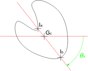 Figure 3. Computation of $R_{min}$ and $R_{max}$ 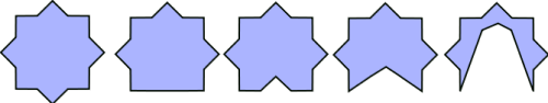 Figure 4. Examples of symmetry measurements In the examples of figure 4, the symmetry factor is from left to right equal to 0.99, 0.879, 0.775, 0.723 and 0.214. |
Floating point | [label] | COEFFICIENT |
| Orientation2d | The 2D orientation of the particle, in degrees in the range [-90,+90], computed from the inertia moments.
The orientation of the largest eigenvalue of the covariance matrix. |
Floating point | [label] | ANGLE |
| Orientation1Phi3d | The polar angle of the particle 3D orientation, in degrees in the range [0,+90], computed from the inertia moments.
It corresponds to the phi orientation of the largest eigenvalue of the covariance matrix. |
Floating point | [label] | ANGLE |
| Orientation1Theta3d | The azimuthal angle of the particle 3D main orientation, in degrees in the range [-180,+180], computed from the inertia moments.
It corresponds to the theta orientation of the largest eigenvalue of the covariance matrix. |
Floating point | [label] | ANGLE |
| Orientation3Phi3d | The polar angle of the particle 3D minor orientation, in degrees in the range [0,+90], computed from the inertia moments.
It corresponds to the phi orientation of the smallest eigenvalue of the covariance matrix. |
Floating point | [label] | ANGLE |
| Orientation3Theta3d | The azimuthal angle of the particle 3D minor orientation, in degrees in the range [-180,+180], computed from the inertia moments.
It corresponds to the theta orientation of the smallest eigenvalue of the covariance matrix. |
Floating point | [label] | ANGLE |
| Euler2d | The Euler2d characteristic, which is a topological invariant indicator. In 2D it corresponds to 1 minus the number of holes.
More information is available in the EulerNumber2d algorithm description. |
Integer | [label] | COUNT |
| Euler3d | The Euler3d characteristic, which is a topological invariant indicator.
More information is available in the EulerNumber3d algorithm description. |
Floating point | [label] | COUNT |
| IntegralMeanCurvature | Computes the integral of mean curvature of objects in a three-dimensional binary image.
More information is available in the CurvatureIntegrals3d algorithm description. |
Floating point | [label] | UNKNOWN |
| IntegralTotalCurvature | Computes the integral of total curvature of objects in a three-dimensional binary image.
More information is available in the CurvatureIntegrals3d algorithm description. |
Floating point | [label] | UNKNOWN |
| NeighborCount | The number of objects close to the current object. It is possible to configure two parameters: Cut-off distance and minimum overlap. This measurement can be used for identifying particles belonging to a cluster.
Let $COD$ be the cut-off distance representing the distance from the boundary of the considered object to the candidate neighbor objects. $COD$ defines a sphere of influence $SOI$. To be counted as a neighbor of the current label $i$, a label $j$ must have a minimum overlap with $SOI(i)$. The overlap $Ov$ is defined by: $$ Ov(i,j) = \frac{Volume(SOI(i)\cap j)}{Volume(j)} $$ where $Volume$ represents the Area2d measurement in 2D, Volume3d in 3D and $\cap$ the intersection operator. 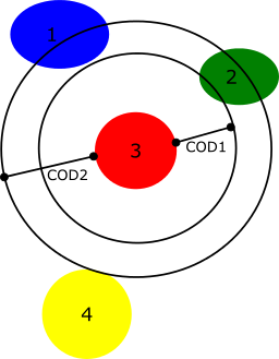 Figure 5. Neighbor counting for label 3 with 3 potential neighbors From the example in figure 5, consider the red particle with label 3 and different attribute configurations, the results are:
The cut-off distance and minimum overlap parameters of this measurement are customizable with the NeighborCount attributes. |
Integer | [label] | COUNT |
Object methods
| Method | Description |
|---|---|
| void toDataFrame() |
Convert the measurement to an IOLink.DataFrame One or more "index" columns will be added at the beginning of the dataframe to identify the different elements. For instance:
|
| Method | Description |
|---|---|
| void ToDataFrame() |
Convert the measurement to an IOLink.DataFrame One or more "index" columns will be added at the beginning of the dataframe to identify the different elements. For instance:
|
| Method | Description |
|---|---|
| void to_data_frame() |
Convert the measurement to an IOLink.DataFrame One or more "index" columns will be added at the beginning of the dataframe to identify the different elements. For instance:
|
© 2026 Thermo Fisher Scientific Inc. All rights reserved.