Edge Marking
This group provides operators for segmenting or sharpening edges.
- ImageLocalMaxima2d: Removes the non-local maxima from the gradient amplitude of a two-dimensional image.
- ImageLocalMaxima3d: Removes the non-local maxima from the gradient amplitude of a three-dimensional image.
- RidgeDetection: Provides the local maxima of an image.
- ZeroCrossings2d: Thresholds pixels where the sign of a Laplacian image changes.
- DijkstraShortestPath2d: Finds the shortest path through an image, considering the image intensities as weights.
- EigenvaluesToStructureness2d: Computes a structure score image from the eigenvalues of a two-dimensional tensor image.
- EigenvaluesToStructureness3d: Computes a structure score image from the eigenvalues of a three-dimensional tensor image.
- TensorVoting2d: Strengthens local features in a two-dimensional image according to their consistency with a model of smooth curves.
- CannyEdgeDetector2d: Performs Canny's computational approach to edge detection on a two-dimensional grayscale image.
- CannyEdgeDetector3d: Performs Canny's computational approach to edge detection on a three-dimensional grayscale image.
Introduction to Edge Marking
With a gradient (for example, GradientMagnitude2d), resp. Laplacian (for example, RecursiveLaplacian2d), operator, a one-dimensional edge is defined as the local maximum of the magnitude of the first derivative, resp. the zero crossing of the second derivative.Gradient Edge Marking
Unfortunately, this definition cannot be extended to two-dimensional or three-dimensional functions. In fact, an edge appears like a crest line on the magnitude of the gradient image and this leads us to define an edge as all the points whose gradient magnitude is maximum along the direction of the gradient (the direction across the edge). This method, referred to as "non-maxima suppression", provides thin lines that are much more convenient to handle.Finally, we can take into account the specific geometry of a contour. Its pixels are connected by using a more sophisticated threshold: the threshold by hysteresis (HysteresisThresholding).
This is in fact an intuitive method. We choose a high and low threshold, $t_h$ and $t_l$, and decide that:
- All pixels having an intensity higher than $t_h$ are edges and thus form the high confidence area,
- Those with intensity lower than $t_l$ are rejected because considered as noise,
- Pixels of the transition area $A$ (for instance, with an intensity lying between $t_l$ and $t_h$) are retained only if they are topologically connected to a pixel of the high confidence area. Two pixels are topologically connected if they belong to the same connected component.
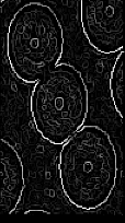
 (a) |
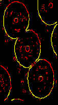
 (b) |
 (c) |
(a) gradient image, (b) classic thresholding does not detect enough edges if threshold is too high (yellow) or reveals noise if too low (red), (c) thresholding by hysteresis
Laplacian Edge Marking
Binary images of Laplacian zero-crossings result in closed thin lines as they correspond to boundaries between positive and negative regions.© 2026 Thermo Fisher Scientific Inc. All rights reserved.