Gradient
This group provides first-order derivative operators.
- GradientOperator2d: Provides different algorithms to perform an edge detection based on the first derivative of a two-dimensional image.
- GradientOperator3d: Provides different algorithms to perform an edge detection based on the first derivative of a three-dimensional image.
- VectorToMagnitude2d: Computes amplitude and orientation of a 2D vector such as a gradient from its X and Y components.
- VectorToMagnitude3d: Computes the amplitude of a 3D vector such as a gradient from its X, Y, and Z components.
- GradientVector2d: Provides different algorithms to perform an edge detection based on the first derivative of a two-dimensional image.
- GradientVector3d: Provides different algorithms to perform an edge detection based on the first derivative of a three-dimensional image.
- GradientMagnitude2d: Provides different algorithms to perform an edge detection based on the first derivative of a two-dimensional image.
- GradientMagnitude3d: Provides different algorithms to perform an edge detection based on the first derivative of a two-dimensional image.
- MorphologicalGradient2d: Approximates an image gradient by using morphological operations.
- MorphologicalGradient3d: Approximates an image gradient by using morphological operations.
- RadialGradientCentered2d: Performs a two-dimensional gradient projection with a directional vector defined by a center point.
- RadialGradientCentered3d: Performs a three-dimensional gradient projection with a directional vector defined by a center point.
- RadialGradientContour2d: Performs a two-dimensional gradient projection with a directional vector defined by a set of contour points of a binary image.
- RadialGradientContour3d: Performs a three-dimensional gradient projection with a directional vector defined by a set of contour points of a binary image.
- RadialGradientLabel2d: Performs a two-dimensional gradient projection with a directional vector defined by a set of object centers of a label image.
- RadialGradientLabel3d: Performs a three-dimensional gradient projection with a directional vector defined by a set of object centers of a label image.
Introduction to Gradient
In the continuous two-dimensional case, the gradient of an image $I(x,y)$ is defined along two orthogonal directions as: $$ G_x(x,y)=\partial I(x,y)/\partial x $$ $$ G_y(x,y)=\partial I(x,y)/\partial y $$ This operator is approximated in the discrete case by differences, as initially introduced by Roberts : $$ \nabla_0(i,j)=I(i,j+1)-I(i,j) $$ $$ \nabla_{90}(i,j)=I(i+1,j)-I(i,j) $$ along horizontal and vertical directions, or: $$ \nabla_{45}(i,j)=I(i+1,j+1)-I(i,j) $$ $$ \nabla_{135}(i,j)=I(i+1,j-1)-I(i,j) $$ along first and second diagonal directions.These operators are implemented by convolutions with the kernels specified in Figure 1. They enhance edges in the {0,90} or {45,135} directions, respectively.
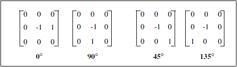
Figure 1. Roberts Gradient Edge Detectors
In addition, one can define the magnitude $G$ and orientation $\Theta$ of the gradient, as: $$ G(i,j)=[\nabla_0^2(i,j)+\nabla_{90}^2(i,j)]^{1/2} ~ \mbox{or} ~ [\nabla_{45}^2(i,j)+; \nabla_{135}^2(i,j)]^{1/2} $$ $$ \Theta(i,j)=\arctan[\nabla_{90}(i,j)/\nabla_0(i,j)] ~ \mbox{or} ~ \arctan[\nabla_{135}(i,j)/; \nabla_{45}(i,j)]+\pi/4 $$ Notice: When applying such filters to an image, the output images consist of positive and negative intensities, with an unusual appearance.
The derivative operator behaves as a high frequency filter; that is, it emphasizes details of an image. An immediate drawback of these gradient filters is their sensitivity to noise. When applied to grainy or textured images, the output image consists of high intensities that correspond to both true edges (luminance transitions), and noise (texture, grain aspect, etc.). This sensitivity to noise can be reduced by using larger kernels to approximate the derivative operators.
Typical masks, such as Prewitt or Sobel detectors for 3x3 kernels are given in Figure 2.
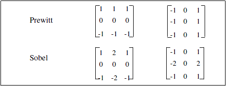
Figure 2. Prewitt and Sobel masks
Another approach is to use morphological operators to estimate the gradient magnitude. We can then define morphological gradients as:
- $D_B(I)-I$ which marks the outer contours,
- $I-E_B(I)$ which marks the inner contours,
- $D_B(I)-E_B(I)$ which marks contours of two-pixel widths for a 3x3 kernel B.
$D_B(I)$ is the result of a dilation with the neighborhood B, and $E_B(I)$ the result of an erosion.
In $R^2$, it can be shown that $\frac{D_B-E_B}{2r}$ tends towards the gradient magnitude when B is a disk whose radius r tends towards 0.
Gradient detection
The output of the above gradients are gray level images, corresponding to emphasized edges in two orthogonal directions. The next step is to identify the pixels on these images that actually correspond to edge points.A common approach is to mark points of sufficiently large gradient magnitude; for instance, points where the luminance transition is sharp enough. This threshold of the gradient magnitude is illustrated in Figure 3.
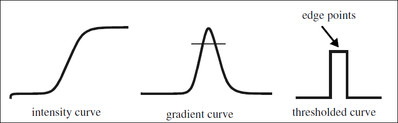
Figure 3. Thresholding a gradient
The overall detection scheme is outlined in Figure 4.
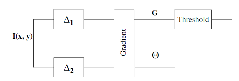
Figure 4. Gradient Computation
Remark: The normalization parameter divides the value of the gradient by the sum of the absolute values of the masks, which reduces the noise sensitivity, avoids overflow, but lowers the contrast. Only main edges will appear on the gradient image. If no normalization is performed, be careful with possible overflow, but edges will be much more evident.
Gradient Projections
In the continuous two-dimensional case, for a given pixel $P$ and knowing the gradient components $G_x$ and $G_y$, the projected gradient $G_C$ of $P$ from the center $C$ is defined along the unitary vector $U(u,v)$, as:$$ G_C=G_x\times u + G_y\times v, ~with~ U(u,v)=\frac{\overrightarrow{P-C} }{\left \| P-C \right \|} $$ In the continuous three-dimensional case, for a given voxel $P$ and knowing the gradient components $G_x$, $G_y$ and $G_z$, the projected gradient $G_C$ of $P$ from the center $C$ is defined along the unitary vector $U(u,v,w)$, as :
$$ G_p=G_x\times u + G_y\times v + G_z\times w, ~with~ U(u,v,w)=\frac{\overrightarrow{P-C} } {\left \| P-C \right \|} $$
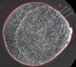 (a) |
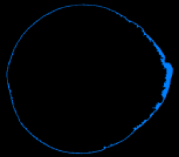 (b) |
(a) input gray level image with contour (red) or single point (blue) defined projection centers, (b) the projected resulting gradient image (Normal Gradient)
The center C can be defined in different ways:
- As a same point for all image pixels/voxels of the input image $I$
- As a set of contour points from which the closest is used as projection center for each point of $I$
- As a set of objects from which the closest barycenter is used as projection center for each point of $I$